Abstract
Wind energy is acknowledged for its status as a renewable energy source that offers several advantages, including its low cost of electricity generation, abundant availability, high efficiency, and minimal environmental impact. The prediction of wind speed using machine learning algorithms is crucial for various applications, such as wind energy planning and urban development. This paper presents a case study on wind speed prediction in Palestine Jerusalem city using the Adaptive Neuro-Fuzzy Inference System (ANFIS) and K-Nearest Neighbors Regression (KNNR) algorithms. The study evaluates their performance using multiple metrics, including root mean square (RMSE), bias, and coefficient of determination R2. ANFIS demonstrates good accuracy with lower RMSE (0.196) and minimal bias (0.0003). However, there is room for improvement in capturing overall variability (R2 = 0.15). In contrast, KNNR exhibits a higher R2 (0.4093), indicating a better fit, but with a higher RMSE (1.4209). These results demonstrated the potential of machine learning algorithms in wind speed prediction, which can lead to optimize the wind energy generation at specific site, and reducing the cost of energy production. This study provides insights into the applicability of ANFIS and KNNR in wind speed prediction for Jerusalem and suggests future research directions. The outcomes have practical implications for wind energy planning, urban development, and environmental assessments in similar regions.
Keywords
Wind Speed, Machine Learning, ANFIS, KNNR
1. Introduction
Accurately predicting wind speed plays a crucial role in many sectors, including renewable energy, maritime, aviation, urban development, agriculture, and environmental assessments. Accurate and reliable predictions of wind speed enable these industries to plan and adjust their activities based on the prevailing wind conditions, ensuring safety and optimal performance
| [1] | M. Madhiarasan, “Accurate prediction of different forecast horizons wind speed using a recursive radial basis function neural network,” Protection and Control of Modern Power Systems, Vol. 5, pp. 22-30, 2020, https://doi.org/10.1186/s41601-020-00166-8 |
[1]
. In recent years, machine learning algorithms have emerged as powerful tools for enhancing the accuracy and reliability of wind speed predictions
| [2] | S. Hanifi, X. Liu, Z. Lin, and S. Lotfian, “A Critical Review of Wind Power Forecasting Methods—Past, Present and Future,” Energies (Basel), Vol. 13, pp. 3764-3788, 2020, https://doi.org/10.3390/en13153764 |
[2]
. This work presents a case study that focuses on predicting wind speed in Jerusalem, utilizing the Adaptive Neuro-Fuzzy Inference System (ANFIS) and K-Nearest Neighbors Regression (KNNR) machine learning algorithms.
The city of Jerusalem, situated in a complex geographical region, experiences diverse wind patterns influenced by factors such as topography, local weather conditions, and seasonal variations. The accurate prediction of wind speed in Jerusalem holds significant importance for the planning and development of wind energy projects, urban infrastructure, and environmental impact assessments.
The implementation of machine learning algorithms in wind speed prediction offers many advantages
. Firstly, these algorithms can effectively extract the hidden patterns by analyzing large datasets. Moreover, through learning from historical data, they can improve prediction accuracy over time. So, they contribute to more informed decision-making processes and more reliable models for wind speed prediction.
The primary objective of this paper is to improve the prediction of wind speed in Jerusalem using ANFIS and KNNR, and to conduct a comparison between ANFIS and KNNR to determine which of both outperforms the other. ANFIS is a Takagi-Sugeno fuzzy inference system implemented as an artificial neural network, making it suitable for handling nonlinear problems and uncertainties
| [4] | J.-S. R. Jang, “Self-Learning Fuzzy Controllers Based on Temporal Backpropagation,” Trans. Neur. Netw., Vol. 3, pp. 714–723, 1992, https://doi.org/10.1109/72.159060 |
[4]
. On the other hand, KNNR is a regression algorithm that predicts values by taking the average of the k nearest neighbors of the target instance
. By implementing these algorithms, we aim to evaluate their performance and effectiveness in accurately predicting wind speed in Jerusalem.
To accomplish this, the machine-learning algorithms underwent training utilizing wind data collected over an extensive timeframe spanning 11 years. To address the presence of empty cells and ensure data completeness, a preprocessing step was executed using the pandas imputing function. The accuracy of the algorithms is evaluated using three evaluation metrics, namely root mean square error (RMSE), coefficient of determination R2 and bias.
The findings of this case study have practical implications for the beforementioned sectors relying on wind speed predictions in Jerusalem. This study evaluates the performance of ANFIS and KNNR, which aids in choosing the most suitable model for wind speed prediction in Jerusalem. Moreover, this research contributes to the existing literature on wind speed prediction In Jerusalem by assessing the performance of ANFIS and KNNR.
In the following sections, we provide some related works, present a detailed analysis of the dataset, describe the methodology employed for training both algorithms, present the results and discuss them. Ultimately, the aim of this case study is to improve wind speed prediction in Jerusalem and inform the selection of suitable models for accurate wind speed forecasting.
2. Related Work
In recent times, the application of machine learning algorithms has witnessed pervasive utilization in the domain of predictive modeling, encompassing the realm of wind speed prediction. This has culminated in substantial advancements surpassing conventional prediction models, thereby manifesting in heightened precision and the extraction of salient features
.
Numerous studies have been carried out to improve local wind speed prediction accuracy and reliability by utilizing machine learning algorithms. This section aims to provide an overview of the existing research, discuss the advantages and limitations of different models, and identify the gaps that this case study seeks to address.
One prevailing machine learning paradigm deployed for the purpose of wind speed prediction is artificial neural networks (ANNs). The framework of an artificial neural network commonly encompasses multiple layers of interconnected nodes, reminiscent of biological neurons, featuring a minimum of one hidden layer, as well as input and output layers. This architectural arrangement enables the ANN to effectively capture intricate non-linear associations between the input variables (inclusive of influential factors such as time, temperature, pressure, among others) and the output variable (wind speed). Such associations are elucidated through a process of training, which has yielded encouraging outcomes. Notably, in a study
, two methods are used for wind prediction: backpropagation neural network and recurrent neural network. The results indicate that neural network prediction outperforms conventional statistical time series analysis in terms of accuracy. Nevertheless, it is worth noting that ANNs frequently necessitate meticulous preprocessing of data and can exhibit sensitivity towards the selection of input features and the design of their architectural structure.
An additional noteworthy approach encompassing wind speed prediction is the employment of the support vector machine (SVM). In
SVM technique was employed to predict wind speed within different time horizons, demonstrating its superiority the radial basis function (RBF) and the persistence model in the very short time horizon. However, it is worth highlighting that SVM may face challenges when with huge datasets and the determination of suitable kernel functions, posing as potential challenges in its application.
In recent years, hybrid models that combine different machine learning algorithms have gained attention. The primary concept behind hybrid models is to integrate different approaches to take advantage of each
. While the primary objective of combining models is typically to enhance prediction accuracy, it is important to note that this approach does not guarantee superior performance compared to the best individual models in all cases. However, combining models is credible because it optimizes information that is limited in the individual models
| [10] | Zhao Dongmei, Zhu Yuchen, and Zhang Xu, “Research on wind power forecasting in wind farms,” IEEE Power Engineering and Automation Conference, pp. 175–178, 2011, https://doi.org/10.1109/PEAM.2011.6134829 |
[10]
. Hybrid models incorporate multiple approaches, such as a mixture of physical and statistical methods or a mixture of short- and medium-term models
| [11] | S. S. Soman, H. Zareipour, O. Malik, and P. Mandal, “A review of wind power and wind speed forecasting methods with different time horizons,” North American Power Symposium, pp. 1–8, 2010, https://doi.org/10.1109/NAPS.2010.5619586 |
[11]
.
Shi et al in
| [12] | J. Shi, J. Guo, and S. Zheng, “Evaluation of hybrid forecasting approaches for wind speed and power generation time series,” Renewable and Sustainable Energy Reviews, Vol. 16, pp. 3471–3480, 2012, https://doi.org/10.1016/j.rser.2012.02.044 |
[12]
present two hybrid models that combine the Autoregressive Integrated Moving Average (ARIMA) method with different techniques. The first hybrid model integrates ARIMA with Artificial Neural Networks (ANN), while the second hybrid model combines ARIMA with Support Vector Machines (SVM). The research investigates the applicability of these hybrid models through two time-horizons. In these models, the ARIMA method is employed to capture linear features, while the other methods are utilized to capture nonlinear features. The empirical results suggest that the novel hybrid models present viable alternatives for forecasting wind speed time series. However, it is crucial to acknowledge that these hybrid approaches do not consistently outperform the individual methods across all prediction time horizons examined in the study.
The fuzzy logic approach employs a nonlinear mapping technique that utilizes linguistic variables (such as low, medium, and high) and a truth variable that ranges from zero to one. This approach is valuable in situations where accurately modeling a system is challenging, but an imprecise model exists. However, it is important to note that relying solely on fuzzy logic is not entirely satisfactory due to its limited learning capability. The ANN-fuzzy technique is a hybrid approach that combines the strengths of artificial neural networks (ANN) and fuzzy logic, where ANN is particularly effective in processing fundamental computations using unprocessed data, while fuzzy logic is better suited for complex computations involving advanced reasoning like human thinking.
In
| [13] | G. Sideratos and N. D. Hatziargyriou, “An Advanced Statistical Method for Wind Power Forecasting,” IEEE Transactions on Power Systems, Vol. 22, pp. 258–265, 2007, https://doi.org/10.1109/TPWRS.2006.889078 |
[13]
, a combination of artificial neural networks (ANN) and a fuzzy logic approach is employed to optimize the utilization of Numerical Weather Predictions (NWPs). The process begins with the ANN model providing an initial wind speed forecast utilizing the NWPs. Subsequently, the fuzzy model assesses the accuracy of the predictions generated by the NWPs. Finally, these evaluations are utilized by an ANN model to generate the final predictions. This integration optimizes the utilization of NWPs and enables the generation of accurate predictions for wind speed by leveraging the strengths of both techniques as confirmed by the simulation results. Nevertheless, fuzzy logic models may require manual rule design and are sensitive to the selection of membership functions.
While the above-mentioned studies have contributed valuable insights, there is only one study that has specifically focused wind speed prediction in the Jerusalem region using machine learning algorithms
| [14] | S. Salah, H. R. Alsamamra, and J. H. Shoqeir, “Exploring Wind Speed for Energy Considerations in Eastern Jerusalem-Palestine Using Machine-Learning Algorithms,” Energies (Basel), Vol. 15, pp. 2602-2618, 2022, https://doi.org/10.3390/en15072602 |
[14]
. Given the unique geographical characteristics and wind patterns of Jerusalem, there is a need for a case study that evaluates the performance of machine learning algorithms tailored to this context.
This study aims to bridge this gap by conducting a comparative analysis of two machine learning algorithms, ANFIS and K-Nearest Neighbors Regression (KNNR), for wind speed prediction in Jerusalem. By specifically examining the performance of these algorithms in the Jerusalem region, this case study seeks to provide valuable insights into the effectiveness of machine learning models for accurately predicting wind speed patterns in this context.
In summary, previous research has explored various machine learning techniques for wind speed prediction, including ANNs, SVM, and hybrid approaches. However, there is a lack of studies focusing on wind speed prediction in Jerusalem using machine learning algorithms. This case study aims to contribute to the existing literature by evaluating the performance of ANFIS and KNNR in capturing the unique wind patterns observed in Jerusalem and providing valuable insights for wind energy planning, urban development, agriculture, and environmental assessments in the region.
3. Materials and Methods
3.1. Modeling
This study adopts a conventional machine learning approach that comprises the following steps: obtaining data, processing data, selecting features, constructing a machine learning model, and evaluating the model through testing and validation.
This scientific investigation presents a meticulous examination into the prediction of wind speed by employing cutting-edge machine learning algorithms. Specifically, this case study delves into the utilization of two prominent techniques, namely the Adaptive Neuro-Fuzzy Inference System (ANFIS) and the k-Nearest Neighbors Regressor (KNNR), to achieve enhanced wind speed forecasting accuracy.
The ANFIS model represents a hybridized framework that amalgamates the capabilities of fuzzy logic and neural networks. By employing fuzzy logic, the model effectively captures and models the inherent uncertainties present within the system, while the neural network component enables learning and optimization processes. ANFIS develops a fuzzy inference system by adaptively adjusting its parameters through the utilization of a hybrid learning algorithm
.
To accomplish wind speed prediction using ANFIS, the following procedural steps are undertaken: a) The collection of wind speed data, encompassing historical wind speed records alongside relevant input parameters (e.g., temperature, pressure). b) Preprocessing of the data by means of input normalization, and subsequent division into training and testing datasets. c) Training of the ANFIS model utilizing the designated training dataset. This entails the model's adjustment of its parameters through the employment of forward and backward passes, thereby optimizing both the fuzzy membership functions and the neural network weights. d) Validation of the trained model via the utilization of the testing dataset, thereby evaluating its performance based on metrics such as mean absolute error (MAE) or root mean square error (RMSE). e) Once the model has been duly validated, it is primed for wind speed prediction by providing the appropriate input variables.
KNNR is a non-parametric algorithm widely adopted for regression tasks. It leverages the concept of proximity, predicting the output of a novel data point by considering its k nearest neighbors within the training dataset. The predicted value is derived from either an average or a weighted average of the target values associated with these nearest neighbors.
To realize wind speed prediction utilizing KNNR, the following sequence of steps is implemented: a) Preparation of the wind speed dataset, encompassing historical wind speed records alongside the corresponding input parameters. b) Normalization of the input variables and partitioning of the dataset into training and testing subsets. c) Training of the KNNR model via its fitting to the training dataset. The model determines the k nearest neighbors by evaluating the distance metric (e.g., Euclidean distance) and subsequently calculates the predicted wind speed as an average of the values attributed to these neighbors. d) Validation of the trained model employing the testing dataset, accompanied by the assessment of its performance utilizing appropriate evaluation metrics. e) Upon successful validation, the trained KNNR model is deployed for wind speed prediction by supplying the pertinent input variables pertaining to the new data point.
3.2. Dataset
The machine-learning algorithms underwent training utilizing wind data sourced from the extensive network of Palestinian meteorological stations. These datasets were meticulously collected over an extensive timeframe spanning 11 years, specifically commencing from January 1, 2008, and concluding on December 31, 2018. To ensure accuracy and representativeness, the wind measurements were meticulously recorded in a continuous manner, employing a cup generator anemometer positioned at a height of 20 meters. Notably, the data acquisition site was Jabal Al-Mukabber, a village located in East Jerusalem, Palestine, with precise geographic coordinates of Latitude 31.7555 N and Longitude 35.2410 E. This specific region stands at an elevation of 720 meters above sea level, guaranteeing a comprehensive and diverse dataset for the subsequent analyses and model training.
The data set contained four features: Time stamp, wind speed, air temperature, and atmospheric pressure. Measurements were taken at 3-hour intervals (8 measurements for each day). The dataset itself consisted of an extensive 32,131 rows of data. Notably, within this dataset, 150 rows were identified to have zero values in the wind speed variable, while an additional 69 rows lacked data, specifically with 36 missing values in the wind speed variable and 33 missing values in the temperature variable.
To address the presence of empty cells and ensure data completeness, a preprocessing step was executed using the pandas imputing function. This essential data manipulation task was accomplished using a Python script, expertly filling the vacant cells with appropriate values. It is worth noting that the existence of zero values in the wind speed variable is deemed acceptable due to the rounding convention associated with wind speed, where values below 0.25 are rounded down to zero.
Table 1 provides an illustrative subset of the dataset, offering a glimpse into the intricate interplay of the various variables. Furthermore,
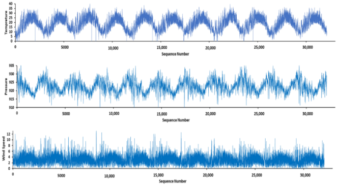
Figure 1 showcases the comprehensive timelines of all variables encapsulated within the dataset, providing a visual representation of their temporal evolution and patterns.
Figure 1. The entire timelines for every variable present in the dataset.
Table 1. A sample of the dataset.
Date | Time | Temperature (°C) | Wind Speed (m/s) | Pressure (mbar) |
25-01-2008 | 8:00 | 5.4 | 3 | 922.8 |
25-01-2008 | 11:00 | 7.9 | 3.5 | 921.6 |
25-01-2008 | 14:00 | 10.7 | 2.5 | 919.7 |
25-01-2008 | 17:00 | 9 | 1 | 919.2 |
25-01-2008 | 20:00 | 8.1 | 0 | 919.5 |
25-01-2008 | 23:00 | 7.3 | 1 | 919.1 |
26-01-2008 | 2:00 | 6.5 | 3 | 918.7 |
A rigorous statistical analysis was conducted on the dataset, yielding insightful findings as presented in
Table 2. It was observed that the wind speed variable exhibited a minimum value of zero, indicating moments of calm conditions, while the maximum value reached 14.5 m/s, denoting instances of heightened wind intensity. The calculated mean wind speed stood at 3.11 m/s, capturing the central tendency of the dataset, while the corresponding standard deviation was determined to be 1.54 m/s, reflecting the dispersion of values around the mean.
Further analysis revealed that three quarters of the wind speed values were found to be less than or equal to 4 m/s. This threshold holds significance, as wind speeds within this range are deemed suitable for the operation of small-scale turbines. Hence, the dataset offers valuable insights into the prevailing wind conditions, suggesting favorable conditions for harnessing wind energy using compact turbine systems.
Regarding the air temperature, it has a mean of 18.22°C and its values range from zero to 39.7°C where three quarters of values are less than 23.4°C. for the atmospheric pressure, values range from 909 to 939.3 mbar while 75% of values are less than 925mbar.
Table 2. The analysis of wind speed data involves calculating various statistical measures such as the minimum, mean, maximum, standard deviation, 25th, 50th, and 75th percentiles of the dataset.
Centralized statistical quantities | Temp (oC) | Pressure (mbar) | Speed (m/s) |
Mean | 18.22 | 922.55 | 3.11 |
SD | 6.98 | 3.67 | 1.54 |
Min | 0 | 909.0 | 0 |
25% | 12.6 | 919.9 | 2.0 |
50% | 18.5 | 922.3 | 3.0 |
75% | 23.4 | 924.9 | 4.0 |
Max | 39.7 | 927.3 | 14.5 |
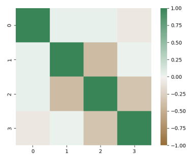
Table 3. Correlation matrix: depicting the correlation coefficients between dataset variables.
| Time | Temperature | Pressure | Speed |
Time | 1 | 0.023 | 0.029 | -0.083 |
Temperature | 0.023 | 1 | -0.415 | 0.009 |
Pressure | 0.029 | -0.415 | 1 | -0.35 |
Speed | -0.083 | 0.009 | -0.35 | 1 |
To analyze the relationships between the variables, the correlations were calculated using the Pearson coefficient. The calculation was done with the Python libraries NumPy and Pandas, the correlation matrix is shown in
Table 3, a heatmap representing the correlation matrix was created with the libraries Matplotlib and Seaborn, it is shown in
Figure 2. In addition, pair plots
Figure 3 between all variables were created using the latter two libraries.
Figure 2. A heat map representing the correlation matrix.
Figure 3. Pair plots displaying pairwise relationships among all variables.
3.3. Evaluation Metrics
The prediction of wind speed inherently encompasses a characteristic element of uncertainty, rendering exactness unattainable. Consequently, it assumes paramount significance to diligently evaluate the accuracy of wind speed predictions. Crucially, the evaluation process necessitates meticulous scrutiny of error measurements utilizing data independent of those employed for model construction or parameter tuning.
By prioritizing comprehensive and unbiased evaluation methodologies, the accuracy and credibility of wind speed predictions can be appropriately assessed, further enhancing the reliability and utility of the predictive models deployed in this domain.
The prediction error is the numerical deviation between the actual measurement and the corresponding prediction, and is mathematically expressed as follows:
Where v_(t+k) represents the actual wind speed (measured value) at a specific moment 't+k', while v ̂_(t+k|t) denotes the predicted wind speed calculated at time ‘t’ for the projected future time ‘t+k’.
It is crucial to assess the accuracy of a predictive model on data that was not utilized in its construction or parameter tuning. Various evaluation metrics, such as Bias Eq (
2), Root Mean Square Error (RMSE) Eq (
2), and coefficient of determination (R
2) Eq (
3) are employed to determine the effectiveness of the model
| [16] | S. Allison, H. Bai, and B. Jayaraman, “Wind estimation using quadcopter motion: A machine learning approach,” Aerosp Sci Technol, Vol. 98, pp. 105699-105712, 2020, https://doi.org/10.1016/j.ast.2020.105699 |
| [17] | H. Madsen, P. Pinson, G. Kariniotakis, H. Aa. Nielsen, and T. S. Nielsen, “Standardizing the Performance Evaluation of Short-Term Wind Power Prediction Models,” Wind Engineering, Vol. 29, pp. 475–489, 2005, https://doi.org/10.1260/030952405776234599 |
[16, 17]
.
(2)
(3)
(4)
Where 'N' denotes the size of the testing sample set, representing the total count of data instances specifically allocated for evaluation and testing purposes within the dataset.
Bias serves as a metric to assess the disparity between the average forecasted wind speed and the actual observed values, indicating overestimation (bias > 0) or underestimation (bias < 0) of the method. However, it only shows systematic errors and lacks information about the forecasting method's accuracy alone
| [18] | Y. Zhao, L. Ye, Z. Li, X. Song, Y. Lang, and J. Su, “A novel bidirectional mechanism based on time series model for wind power forecasting,” Appl Energy, Vol. 177, pp. 793–803, 2016, https://doi.org/10.1016/j.apenergy.2016.03.096 |
[18]
.
Mean Squared Error (MSE) quantifies the average squared disparity between the observed and predicted values, quantifying the model's error. It would be zero in an ideal scenario with 100% accuracy. RMSE considers both random and systematic errors, where larger values indicate greater deviations and smaller values indicate more precise predictions. Significant discrepancies between MAE and RMSE values suggest a wider spread of predicted values in comparison to the measured data
| [18] | Y. Zhao, L. Ye, Z. Li, X. Song, Y. Lang, and J. Su, “A novel bidirectional mechanism based on time series model for wind power forecasting,” Appl Energy, Vol. 177, pp. 793–803, 2016, https://doi.org/10.1016/j.apenergy.2016.03.096 |
[18]
.
R2 is a coefficient of determination indicating the amount of variance explained by the prediction model, with values close to 1 indicating an optimal model and negative values indicating a poor prediction.
4. Results and Discussion
Two machine-learning algorithms were applied on the dataset to predict wind speed, which are adaptive (ANFIS), and k nearest neighbor’s regression (KNNR). The simulation testbed used Intel (R) Core (TM) i7-1265H CPU running @ 2.3 GHz, with 16 GB memory, 64-bit MS Windows 10 Home with x64 processor architecture, The Python environment setup consisted of Python (3.8.11) and common ML libraries, mainly scikit-learn (0.24.2), SKFuzzy and NumPy, among other libraries for data extraction and visualization, such as seaborn and matplotlib. The dataset was split into training and testing sets, 80% (28,017) and 20% (3214) from 2008 to 2018, respectively. This section demonstrates and discusses the results of each model, then A comparison between the two models is conducted. Finally, a comparison between this study and other studies is conducted.
4.1. ANFIS
Several ANFIS experiments were conducted by varying different parameters to search for the optimal model. The experiments involved testing different numbers of membership functions (one, two, and three) for each feature, as well as different epochs, number of populations, and membership functions. Results were analyzed and discussed for each variation.
The evaluation metrics showed that there wasn't a significant difference between using one membership function and three membership functions (RMSE is 0.198 for both). However, using two membership functions resulted in even better results than both one and three, so it was selected as the optimal number of membership functions.
When two membership functions are used for each feature, it usually involves creating two fuzzy sets, with one corresponding to low values and the other to high values. The shapes of these fuzzy sets can vary and may be triangular, trapezoidal, or Gaussian, among others, depending on the data and the specific problem being analyzed. For this problem, the generalized bell function was used for its simplicity and performance.
Four variations of rules were used in this scenario, where the form of the rule is "if [feature1] is low (high) and [feature2] is low (high), then [output] is equal to [coefficients]". For example, one rule might be "if temperature is low and pressure is low, then wind speed is equal to
(5)
The dataset, which contains 32,131 samples, was divided into two sets: 30% for testing (9,640 samples) and 70% for training (22,491 samples). The ANFIS model used four premise membership functions, resulting in 24 parameters. The root mean square error (RMSE) for the training set was 0.193, while the RMSE for the testing set was 0.196.
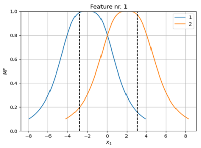
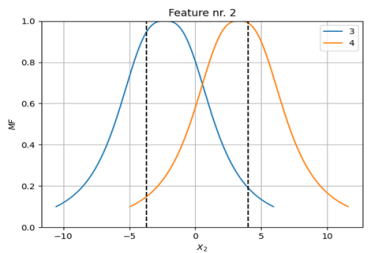
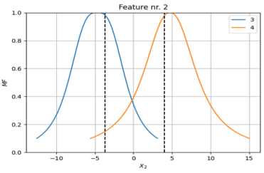
Figures 4 and 5 show the membership functions for the temperature feature before (with mu = -2.9 and std = 3.08) and after (with mu = -2.0 and std = 3.09) modeling, respectively. Similarly,
Figures 6 and 7 depict the membership functions for the pressure feature before (with mu = -4.24 and std = 3.89) and after (with mu = -4.7 and std = 3.8) modeling, respectively, demonstrating changes in the statistical properties of the features due to the modeling process.
Figure 4. The membership functions for the temperature feature before modeling.
Figure 5. the membership functions for the temperature feature after modeling.
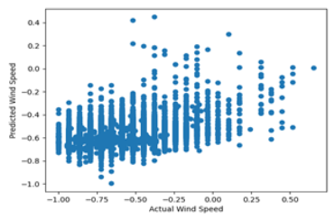
The ANFIS algorithm's prediction visualization is depicted in
Figure 8, where it compares the predicted and actual wind speed values. The visualization revealed a discernible pattern in the ANFIS algorithm's predictions, supporting the recently mentioned accuracy measure (RMSE 0.193), although a few small outliers were visible. According to
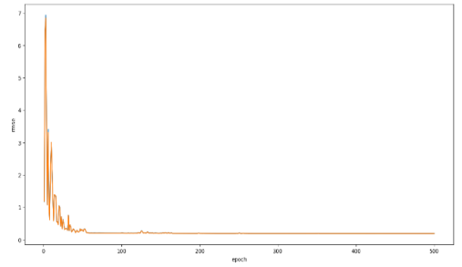
Figure 9, the root mean square error (RMSE) of the ANFIS model decreases significantly before 60 epochs, after which it approaches a horizontal asymptote of approximately 0.12.
Figure 6. The membership functions for the pressure feature before modeling.
Figure 7. The membership functions for the pressure feature after modeling.
Figure 8. The ANFIS algorithm's prediction visualization (predicted wind speed vs actual).
Figure 9. The RMSE of the ANFIS model per epoch.
Bias and R2 values were computed, yielding a bias value of 0.0003 and an R2 value of 0.15. A bias of 0.0003 implies a close correspondence between the predicted and observed wind speed values on average. A negligible bias suggests the absence of systematic overestimation or underestimation of wind speed by the model.
Furthermore, an RMSE value of 0.196 indicates a relatively small average prediction error. RMSE quantifies the average disparity between the predicted and actual wind speed values, with lower values indicating enhanced predictive accuracy. When considering these evaluation metrics together, a bias close to zero and a low RMSE suggest that the model is performing well in terms of predicting wind speed. However, the low R2 value of 0.15 implies that the predicted values account for only a small fraction of the observed wind speed data's variability. This suggests the potential presence of unaccounted factors or variables influencing wind speed.
4.2. KNNR
Several experiments were performed to find the optimal model for KNNR, with different parameters used for each experiment. The variations included changing the number of neighbors, the type of metric used, and the weight function used in prediction. The results for each variation were analyzed and discussed.
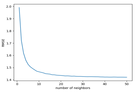
In
Figures 10 and 11, the correlation between the root mean square error (RMSE) and the number of neighbors (k) is illustrated. Specifically,
Figure 10 demonstrates this relationship when the weight function used is "distance", and the metric utilized is the Minkowskian metric with a power of two (also known as the Euclidean metric). On the other hand,
Figure 11 depicts the same relationship but with the "uniform" weight function replacing the "distance" function. In both figures, the root mean square error (RMSE) initially begins at a high value of approximately two, then gradually decreases until it approaches a horizontal asymptote. In
Figure 10, the RMSE approaches an asymptote of approximately 1.66, while in
Figure 11, it approaches an asymptote of approximately 1.42.
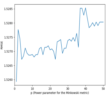
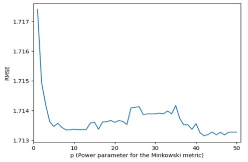
Figures 12 and 13, illustrates the relationship between the root mean square error (RMSE) and the Power parameter for the Minkowski metric (p).
Figure 12 shows this relationship when the weight function used is "distance," and the number of neighbors (k) is 5.
Figure 13 displays the same relationship but with the "uniform" weight function replacing the "distance" function.
Figure 10. The RMSE of the KNNR model vs the number of neighbors (“distance” weight function, p equals 2).
Figure 11. The RMSE of the KNNR model vs the number of neighbors (“uniform” weight function, p equals 2).
In
Figure 12, the RMSE oscillates between p=5 to p=38. Generally, the RMSE increases with an increase in power. Therefore, the best values are at small powers, particularly at p=1 and p=2. On the other hand, in
Figure 13, the RMSE generally decreases as the power increases, except for the interval between p=20 to p=40.
Figure 12. The RMSE of the KNNR model vs the power parameter for the Minkowski metric (“distance” weight function, k equals 5).
Figure 13. The RMSE of the KNNR model vs the Power parameter for the Minkowski metric (“uniform” weight function, k equals 5).
Overall, there is a small difference between the RMSE values in both figures, indicating that choosing the Power parameter for the Minkowski metric (p) is not a significant issue.
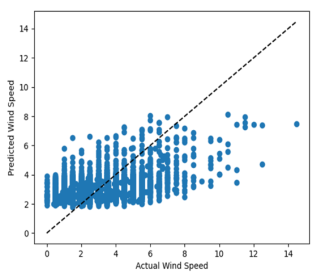
In
Figure 14, the prediction visualization of the KNNR algorithm compares the actual and predicted wind speed values. The results showed that the algorithm struggled to predict high wind speeds since they were infrequent and represented only a small percentage of neighbors for each data point. This finding supports the high RMSE accuracy measure of 1.42 mentioned earlier.
Figure 14. The KNNR algorithm's prediction visualization (predicted wind speed vs actual).
The RMSE value of 1.4209 indicates a relatively higher average prediction error compared to the ANFIS model. A higher RMSE suggests that the KNNR model's predictions have larger deviations from the actual observed wind speed values.
The R2 value of 0.4093 suggests that approximately 40.93% of the variance in the observed wind speed values is explained by the predicted values. Although it is an improvement compared to the ANFIS model, the R2 value still indicates that a significant portion of the variability in the wind speed data remains unexplained by the KNNR model.
The bias value of 0.0369 indicates a slight overall tendency of the KNNR model to slightly overestimate the wind speed values on average. However, the bias is relatively small and close to zero, suggesting that the model's overall tendency to overestimate or underestimate the wind speed is minimal.
When comparing these metrics to the ANFIS model, the KNNR model exhibits a higher RMSE, indicating larger prediction errors. However, the KNNR model has a higher R2 value, suggesting a better fit to the observed wind speed data compared to the ANFIS model. The bias for the KNNR model is slightly higher than that of the ANFIS model but remains relatively small. Additionally, the ANFIS model generated a denser prediction compared to the KNNR model.
Compared to the article by
| [14] | S. Salah, H. R. Alsamamra, and J. H. Shoqeir, “Exploring Wind Speed for Energy Considerations in Eastern Jerusalem-Palestine Using Machine-Learning Algorithms,” Energies (Basel), Vol. 15, pp. 2602-2618, 2022, https://doi.org/10.3390/en15072602 |
[14]
, which employed six machine learning models using the same dataset, the ANFIS model showed lower RMSE values (0.193) than all six models. The RMSE values for the six models were MLR (1.37), Ridge (1.38), Lasso (1.37), Random Forest (1.16), SVR (1.38), and LSTM (1.21).
5. Conclusions
This study investigated the use of machine learning algorithms for wind speed prediction using a dataset collected from a Palestinian meteorological station. The study focused on two popular algorithms: Adaptive Neuro-Fuzzy Inference System (ANFIS) and K-Nearest Neighbor Regression (KNNR). The results obtained from our experiments indicate that both ANFIS and KNNR have their strengths and limitations. ANFIS demonstrated relatively lower RMSE and bias, indicating good accuracy and minimal systematic error in wind speed prediction. However, its R2 value was relatively low, suggesting that there is still room for improvement in capturing the overall variability in the observed wind speed data. On the other hand, KNNR exhibited a higher R2 value, indicating a better fit to the data, although it had a higher RMSE compared to ANFIS. The bias for both algorithms was relatively small.
There are several potential areas for future research in wind speed prediction using machine learning algorithms. The following directions could enhance the accuracy and effectiveness of wind speed models: Exploration of Deep Learning Models, incorporation of Wind Speed Direction, and Extraction of Seasonal and Diurnal Patterns.
Abbreviations
ANFIS | Adaptive Neuro-Fuzzy Inference System |
ANN | Artificial Neural Network |
ARIMA | Auto Regressive Integrated Moving Average |
KNNR | K-Nearest Neighbors Regression |
MAE | Mean Absolute Error |
NWP | Numerical Weather Prediction |
SVM | Support Vector Machine |
Conflicts of Interest
The authors declare no conflicts of interest.
References
| [1] |
M. Madhiarasan, “Accurate prediction of different forecast horizons wind speed using a recursive radial basis function neural network,” Protection and Control of Modern Power Systems, Vol. 5, pp. 22-30, 2020,
https://doi.org/10.1186/s41601-020-00166-8
|
| [2] |
S. Hanifi, X. Liu, Z. Lin, and S. Lotfian, “A Critical Review of Wind Power Forecasting Methods—Past, Present and Future,” Energies (Basel), Vol. 13, pp. 3764-3788, 2020,
https://doi.org/10.3390/en13153764
|
| [3] |
D. Bzdok, N. Altman, and M. Krzywinski, “Statistics versus machine learning,” Nat Methods, Vol. 15, pp. 233–234, 2018,
https://doi.org/10.1038/nmeth.4642
|
| [4] |
J.-S. R. Jang, “Self-Learning Fuzzy Controllers Based on Temporal Backpropagation,” Trans. Neur. Netw., Vol. 3, pp. 714–723, 1992,
https://doi.org/10.1109/72.159060
|
| [5] |
D. Coomans and D. L. Massart, “Alternative k-nearest neighbour rules in supervised pattern recognition”, Anal Chim Acta, Vol. 136, pp. 15–27, 1982,
https://doi.org/10.1016/S0003-2670(01)95359-0
|
| [6] |
S. Mathew, K. P. Pandey, and A. Kumar. V, “Analysis of wind regimes for energy estimation”, Renew Energy, Vol. 25, pp. 381–399, 2002,
https://doi.org/10.1016/S0960-1481(01)00063-5
|
| [7] |
A. More and M. C. Deo, “Forecasting wind with neural networks”, Marine Structures, Vol. 16, pp. 35–49, 2003,
https://doi.org/10.1016/S0951-8339(02)00053-9)
|
| [8] |
J. Zeng and W. Qiao, “Support vector machine-based short-term wind power forecasting”, IEEE/PES Power Systems Conference and Exposition, pp. 1–8, 2011,
https://doi.org/10.1109/PSCE.2011.5772573
|
| [9] |
Y.-K. Wu and J.-S. Hong, “A literature review of wind forecasting technology in the world,” IEEE Lausanne Power Tech, pp. 504–509, 2007,
https://doi.org/10.1109/PCT.2007.4538368
|
| [10] |
Zhao Dongmei, Zhu Yuchen, and Zhang Xu, “Research on wind power forecasting in wind farms,” IEEE Power Engineering and Automation Conference, pp. 175–178, 2011,
https://doi.org/10.1109/PEAM.2011.6134829
|
| [11] |
S. S. Soman, H. Zareipour, O. Malik, and P. Mandal, “A review of wind power and wind speed forecasting methods with different time horizons,” North American Power Symposium, pp. 1–8, 2010,
https://doi.org/10.1109/NAPS.2010.5619586
|
| [12] |
J. Shi, J. Guo, and S. Zheng, “Evaluation of hybrid forecasting approaches for wind speed and power generation time series,” Renewable and Sustainable Energy Reviews, Vol. 16, pp. 3471–3480, 2012,
https://doi.org/10.1016/j.rser.2012.02.044
|
| [13] |
G. Sideratos and N. D. Hatziargyriou, “An Advanced Statistical Method for Wind Power Forecasting,” IEEE Transactions on Power Systems, Vol. 22, pp. 258–265, 2007,
https://doi.org/10.1109/TPWRS.2006.889078
|
| [14] |
S. Salah, H. R. Alsamamra, and J. H. Shoqeir, “Exploring Wind Speed for Energy Considerations in Eastern Jerusalem-Palestine Using Machine-Learning Algorithms,” Energies (Basel), Vol. 15, pp. 2602-2618, 2022,
https://doi.org/10.3390/en15072602
|
| [15] |
J.-S. R. Jang, “ANFIS: adaptive-network-based fuzzy inference system,” IEEE Trans Syst Man Cybern, Vol. 23, pp. 665–685, 1993,
https://doi.org/10.1109/21.256541
|
| [16] |
S. Allison, H. Bai, and B. Jayaraman, “Wind estimation using quadcopter motion: A machine learning approach,” Aerosp Sci Technol, Vol. 98, pp. 105699-105712, 2020,
https://doi.org/10.1016/j.ast.2020.105699
|
| [17] |
H. Madsen, P. Pinson, G. Kariniotakis, H. Aa. Nielsen, and T. S. Nielsen, “Standardizing the Performance Evaluation of Short-Term Wind Power Prediction Models,” Wind Engineering, Vol. 29, pp. 475–489, 2005,
https://doi.org/10.1260/030952405776234599
|
| [18] |
Y. Zhao, L. Ye, Z. Li, X. Song, Y. Lang, and J. Su, “A novel bidirectional mechanism based on time series model for wind power forecasting,” Appl Energy, Vol. 177, pp. 793–803, 2016,
https://doi.org/10.1016/j.apenergy.2016.03.096
|
Cite This Article
-
APA Style
Abuayyash, K., Alsamamra, H., Teir, M. A., Doufesh, H. (2024). Wind Speed Prediction in Jerusalem Using Machine Learning Algorithms: A Case Study of Using ANFIS and KNNR. American Journal of Modern Energy, 10(2), 25-37. https://doi.org/10.11648/j.ajme.20241002.12
 Copy
|
Copy
|
 Download
ACS Style
Abuayyash, K.; Alsamamra, H.; Teir, M. A.; Doufesh, H. Wind Speed Prediction in Jerusalem Using Machine Learning Algorithms: A Case Study of Using ANFIS and KNNR. Am. J. Mod. Energy 2024, 10(2), 25-37. doi: 10.11648/j.ajme.20241002.12
Copy
|
Download
AMA Style
Abuayyash K, Alsamamra H, Teir MA, Doufesh H. Wind Speed Prediction in Jerusalem Using Machine Learning Algorithms: A Case Study of Using ANFIS and KNNR. Am J Mod Energy. 2024;10(2):25-37. doi: 10.11648/j.ajme.20241002.12
Copy
|
Download
-
@article{10.11648/j.ajme.20241002.12,
  author = {Khalil Abuayyash and Husain Alsamamra and Musa Abu Teir and Hazem Doufesh},
  title = {Wind Speed Prediction in Jerusalem Using Machine Learning Algorithms: A Case Study of Using ANFIS and KNNR
},
  journal = {American Journal of Modern Energy},
  volume = {10},
  number = {2},
  pages = {25-37},
  doi = {10.11648/j.ajme.20241002.12},
  url = {https://doi.org/10.11648/j.ajme.20241002.12},
  eprint = {https://article.sciencepublishinggroup.com/pdf/10.11648.j.ajme.20241002.12},
  abstract = {Wind energy is acknowledged for its status as a renewable energy source that offers several advantages, including its low cost of electricity generation, abundant availability, high efficiency, and minimal environmental impact. The prediction of wind speed using machine learning algorithms is crucial for various applications, such as wind energy planning and urban development. This paper presents a case study on wind speed prediction in Palestine Jerusalem city using the Adaptive Neuro-Fuzzy Inference System (ANFIS) and K-Nearest Neighbors Regression (KNNR) algorithms. The study evaluates their performance using multiple metrics, including root mean square (RMSE), bias, and coefficient of determination R2. ANFIS demonstrates good accuracy with lower RMSE (0.196) and minimal bias (0.0003). However, there is room for improvement in capturing overall variability (R2 = 0.15). In contrast, KNNR exhibits a higher R2 (0.4093), indicating a better fit, but with a higher RMSE (1.4209). These results demonstrated the potential of machine learning algorithms in wind speed prediction, which can lead to optimize the wind energy generation at specific site, and reducing the cost of energy production. This study provides insights into the applicability of ANFIS and KNNR in wind speed prediction for Jerusalem and suggests future research directions. The outcomes have practical implications for wind energy planning, urban development, and environmental assessments in similar regions.
},
 year = {2024}
}
Copy
|
Download
-
TY  - JOUR
T1  - Wind Speed Prediction in Jerusalem Using Machine Learning Algorithms: A Case Study of Using ANFIS and KNNR

AU  - Khalil Abuayyash
AU  - Husain Alsamamra
AU  - Musa Abu Teir
AU  - Hazem Doufesh
Y1  - 2024/05/30
PY  - 2024
N1  - https://doi.org/10.11648/j.ajme.20241002.12
DO  - 10.11648/j.ajme.20241002.12
T2  - American Journal of Modern Energy
JF  - American Journal of Modern Energy
JO  - American Journal of Modern Energy
SP  - 25
EP  - 37
PB  - Science Publishing Group
SN  - 2575-3797
UR  - https://doi.org/10.11648/j.ajme.20241002.12
AB  - Wind energy is acknowledged for its status as a renewable energy source that offers several advantages, including its low cost of electricity generation, abundant availability, high efficiency, and minimal environmental impact. The prediction of wind speed using machine learning algorithms is crucial for various applications, such as wind energy planning and urban development. This paper presents a case study on wind speed prediction in Palestine Jerusalem city using the Adaptive Neuro-Fuzzy Inference System (ANFIS) and K-Nearest Neighbors Regression (KNNR) algorithms. The study evaluates their performance using multiple metrics, including root mean square (RMSE), bias, and coefficient of determination R2. ANFIS demonstrates good accuracy with lower RMSE (0.196) and minimal bias (0.0003). However, there is room for improvement in capturing overall variability (R2 = 0.15). In contrast, KNNR exhibits a higher R2 (0.4093), indicating a better fit, but with a higher RMSE (1.4209). These results demonstrated the potential of machine learning algorithms in wind speed prediction, which can lead to optimize the wind energy generation at specific site, and reducing the cost of energy production. This study provides insights into the applicability of ANFIS and KNNR in wind speed prediction for Jerusalem and suggests future research directions. The outcomes have practical implications for wind energy planning, urban development, and environmental assessments in similar regions.

VL  - 10
IS  - 2
ER  -
Copy
|
Download